Content from What is OMOP?
Last updated on 2026-02-08 | Edit this page
Overview
Questions
- What is OMOP?
- Why is using a standard important in healthcare data?
- How do OMOP tables relate to each other?
- What are concept_ids and how can we get an humanly readable name for them?
Objectives
- Examine the diagram of the OMOP tables and the data specification
- Understand OMOP standardization and vocabularies
- Connect to an OMOP database and explore the
concepttable - Get a humanly readable name for a concept_id
Setting up R
Getting started
The “Projects” interface in RStudio not only creates a working directory for you, but also remembers its location (allowing you to quickly navigate to it). The interface also (optionally) preserves custom settings and open files to make it easier to resume work after a break.
Connect to a database
For this episode we will be using the CDMConnector
package to connect to an OMOP Common Data Model database. We define a
function that will open this package and connect an appropriate dataset.
It is listed below but you will also find it in the
workshop/code/CDMConnector directory that you should have
downloaded. This package also contains synthetic example data that can
be used to demonstrate querying the data.
R
# Libraries
library(CDMConnector)
library(DBI)
library(duckdb)
library(dplyr)
library(dbplyr)

# Connect to GiBleed if not already connected
if (!exists("cdm") || !inherits(cdm, "cdm_reference")) {
  db_name <- "GiBleed"
  CDMConnector::requireEunomia(datasetName = db_name)
  con <- DBI::dbConnect(duckdb::duckdb(),
                        dbdir = CDMConnector::eunomiaDir(datasetName = db_name))
  cdm <- CDMConnector::cdmFromCon(con, cdmSchema = "main", writeSchema = "main")
}
OUTPUT
Download completed!Introduction
OMOP is a format for recording Electronic Healthcare Records. It allows you to follow a patient journey through a hospital by linking every aspect to a standard vocabulary thus enabling easy sharing of data between hospitals, trusts and even countries.
OMOP CDM Diagram
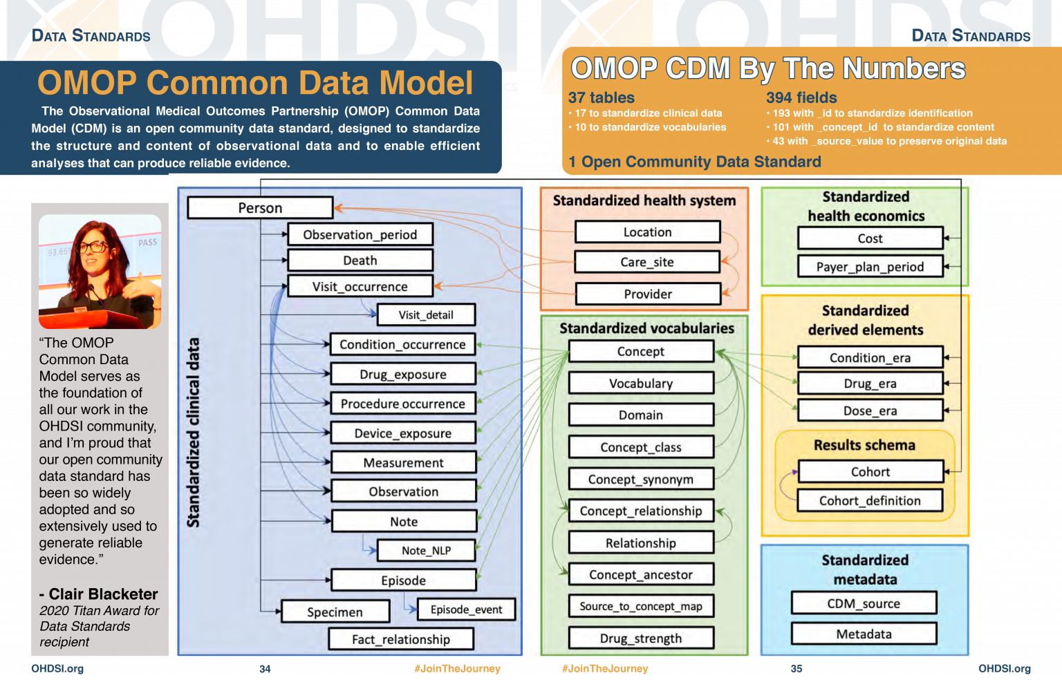
OMOP CDM stands for the Observational Medical Outcomes Partnership Common Data Model. You don’t really need to remember what OMOP stands for. Remembering that CDM stands for Common Data Model can help you remember that it is a data standard that can be applied to different data sources to create data in a Common (same) format. The table diagram will look confusing to start with but you can use data in the OMOP CDM without needing to understand (or populate) all 37 tables.
Challenge
Look at the OMOP-CDM figure and answer the following questions:
Which table is the key to all the other tables?
Which table allows you to distinguish between different stays in hospital?
The Person table
The Visit_occurrence table
Why use OMOP?
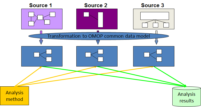
Once a database has been converted to the OMOP CDM, evidence can be generated using standardized analytics tools. This means that different tools can also be shared and reused. So using OMOP can help make your research FAIR.
Read in the database as above.
The data themselves are not actually read into the created cdm object. Rather it is a reference that allows us to query the data from the database.
Typing names(cdm) will give a summary of the tables in
the database and we can look at these individually using the
$ operator and the colnames command.
OMOP Tables
R
names(cdm)
OUTPUT
 [1] "person"                "observation_period"    "visit_occurrence"
 [4] "visit_detail"          "condition_occurrence"  "drug_exposure"
 [7] "procedure_occurrence"  "device_exposure"       "measurement"
[10] "observation"           "death"                 "note"
[13] "note_nlp"              "specimen"              "fact_relationship"
[16] "location"              "care_site"             "provider"
[19] "payer_plan_period"     "cost"                  "drug_era"
[22] "dose_era"              "condition_era"         "metadata"
[25] "cdm_source"            "concept"               "vocabulary"
[28] "domain"                "concept_class"         "concept_relationship"
[31] "relationship"          "concept_synonym"       "concept_ancestor"
[34] "source_to_concept_map" "drug_strength"
Looking at the column names in each table
R
colnames(cdm$person)
OUTPUT
 [1] "person_id"                   "gender_concept_id"
 [3] "year_of_birth"               "month_of_birth"
 [5] "day_of_birth"                "birth_datetime"
 [7] "race_concept_id"             "ethnicity_concept_id"
 [9] "location_id"                 "provider_id"
[11] "care_site_id"                "person_source_value"
[13] "gender_source_value"         "gender_source_concept_id"
[15] "race_source_value"           "race_source_concept_id"
[17] "ethnicity_source_value"      "ethnicity_source_concept_id"
Challenge
How do you think the visit_occurrence table is used to
connect to the person table?
R
colnames(cdm$visit_occurrence)
OUTPUT
 [1] "visit_occurrence_id"           "person_id"
 [3] "visit_concept_id"              "visit_start_date"
 [5] "visit_start_datetime"          "visit_end_date"
 [7] "visit_end_datetime"            "visit_type_concept_id"
 [9] "provider_id"                   "care_site_id"
[11] "visit_source_value"            "visit_source_concept_id"
[13] "admitting_source_concept_id"   "admitting_source_value"
[15] "discharge_to_concept_id"       "discharge_to_source_value"
[17] "preceding_visit_occurrence_id"
Looking at both tables we can see that they both have a column
labelled person_id which could be used to link them
together.
Notice that the visit_concept_id column in the
visit_occurrence table is also a concept_id. This
concept_id can be used to find out more information about the type of
visit (e.g. inpatient, outpatient etc) by looking it up in the
concept table. In this case the
visit_concept_id is 9201 which relates to an inpatient
visit. We can find this out by filtering the concept table
for concept_id 9201 and selecting the
concept_name column.
R
cdm$concept |>
  filter(concept_id == 9201) |>
  select(concept_name)
OUTPUT
# Source:   SQL [?? x 1]
# Database: DuckDB 1.4.1 [unknown@Linux 6.8.0-1044-azure:R 4.5.2//tmp/RtmpY0FW18/file17431739c2fc.duckdb]
  concept_name
  <chr>
1 Inpatient VisitCODING_NOTE: We use filter to identify
the row we want and select to choose the column we want.
This is because we are querying a remote database, not one that is
local. If we were working with a local database we could just use
cdm$concept$concept_name[cdm$concept$concept_id == 9201] to
get the same result.
A useful function
Finding the humanly readable name for a concept_id will
be a useful function. We can create a function
get_concept_name() that takes a concept_id as
input and returns the concept_name.
Challenge
Create the function get_concept_name() that takes a
concept_id as input and returns the
concept_name.
R
get_concept_name <- function(id) {
  cdm$concept |>
    filter(concept_id == !!id) |>
    select(concept_name) |>
    pull()
}
Explanation of function code
- The function is called
get_concept_nameand it takes one argument,id. - Inside the function, we query the
concepttable from thecdmobject. - We use the
filterfunction to select rows where theconcept_idmatches the inputid. The!!operator is used to unquote the variable so that its value is used in the filter. - We then use
selectto choose only theconcept_namecolumn from the filtered results. - Finally, we use
pull()to extract theconcept_nameas a vector, which is returned by the function. We need to use this because we are querying a remote database, not one that is local.
Other useful tables
There are also other tables which will give you other information about concepts.
R
colnames(cdm$concept)
OUTPUT
 [1] "concept_id"       "concept_name"     "domain_id"        "vocabulary_id"
 [5] "concept_class_id" "standard_concept" "concept_code"     "valid_start_date"
 [9] "valid_end_date"   "invalid_reason"
R
colnames(cdm$domain)
OUTPUT
[1] "domain_id" "domain_name" "domain_concept_id"R
colnames(cdm$vocabulary)
OUTPUT
[1] "vocabulary_id"         "vocabulary_name"       "vocabulary_reference"
[4] "vocabulary_version" "vocabulary_concept_id"- Using a standard makes it much easier to share data
- OMOP uses concepts to link different tables together
- The
concepttable contains humanly readable names for concept_ids
Content from Exploring OMOP concepts with R
Last updated on 2026-02-08 | Edit this page
Overview
Questions
- Find the
vocabulary,domainandconcept_classfor a givenconcept_id - Establish whether a
concept_idis a standard concept - Find all concepts within a given domain
- Find all concepts within a given vocabulary
Objectives
- Understand that concepts have additional attributes such as vocabulary, domain, classand standard concept status
- Use R to query the
concepttable for specific attributes of concepts - Filter concepts based on domain, vocabulary and class
- Identify standard concepts within the OMOP vocabulary
Introduction
The primary purpose of the concept table is to provide a
standardised representation of medical Concepts, allowing for consistent
querying and analysis across healthcare databases. Users can join the
concept table with other tables in the CDM to enrich
clinical data with Concept information or use the concept
table as a reference for mapping clinical data from source terminologies
to Standard or other Concepts.
An OMOP concept_id is a unique integer identifier.
Concept_ids are defined in the OMOP concept table where a
corresponding name and other attributes are stored. OMOP contains
concept_ids for other medical vocabularies such as SNOMED and LOINC,
which OMOP terms as source vocabularies.
Nearly everything in a hospital can be represented by an OMOP
concept_id.
Looking up OMOP concepts
OMOP concepts can be looked up in Athena an online tool provided by OHDSI.
The CDMConnector package allows connection to an OMOP Common Data Model in a database. It also contains synthetic example data that can be used to demonstrate querying the data.
In the previous episode we set up the CDMConnector package to connect
to an OMOP Common Data Model database and used it to look at the
concepts table. We also created the function
get_concept_name() to get a humanly readable name for a
concept_id. We will use these again in this episode.
Setting up the connection
R
library(CDMConnector)

db_name <- "GiBleed"
CDMConnector::requireEunomia(datasetName = db_name)
OUTPUT
Download completed!R
db <- DBI::dbConnect(duckdb::duckdb(),
                     dbdir = CDMConnector::eunomiaDir(datasetName = db_name))

cdm <- CDMConnector::cdmFromCon(con = db, cdmSchema = "main",
                                writeSchema = "main")
Exploring the concept table
R
colnames(cdm$concept)
OUTPUT
 [1] "concept_id"       "concept_name"     "domain_id"        "vocabulary_id"
 [5] "concept_class_id" "standard_concept" "concept_code"     "valid_start_date"
[9] "valid_end_date" "invalid_reason" | concept table columns | Description |
|---|---|
| concept_id | Unique identifier for the concept. |
| concept_name | Name or description of the concept. |
| domain_id | The domain to which the concept belongs (e.g. Condition, Drug). |
| vocabulary_id | The vocabulary from which the concept originates (e.g. SNOMED, RxNorm). |
| concept_class_id | Classification within the vocabulary (e.g. Clinical Finding, Ingredient). |
| standard_concept | ‘S’ for standard concepts that come from internationally accepted standard vocabularies. |
| concept_code | Code used by the source vocabulary to identify the concept. |
| valid_start_date | Date the concept became valid in OMOP. |
| valid_end_date | Date the concept ceased to be valid. |
| invalid_reason | Reason for invalidation, if applicable |
The concept table is the main table for looking up
information about concepts. We can use R to query the
concept table for specific attributes of concepts.
Challenge
Answer the following questions using R and the concept
table:
How many entries are there in the
concepttable?How many distinct vocabularies are there in the
concepttable?How many distinct domains other than ‘None’ are there in the
concepttable?How many distinct concept_classes are there in the
concepttable?
- How many entries are there in the
concepttable?
R
library(dplyr)
cdm$concept |>
  summarise(n_concepts = n())
OUTPUT
# Source:   SQL [?? x 1]
# Database: DuckDB 1.4.1 [unknown@Linux 6.8.0-1044-azure:R 4.5.2//tmp/Rtmpd8tQ6t/file17767ba676cb.duckdb]
  n_concepts
       <dbl>
1        444
Answer: There are 444 entries in the
concept table. This is a tiny fraction of the overall table
which can be found at Athena
CODING_NOTE: The function n() counts
the number of rows in the table and summarise() creates a
summary table with that count. These functions are part of the
dplyr package. When you have loaded the library once your
environment will remember it for the rest of the session.
- How many distinct vocabularies are there in the
concepttable?
R
cdm$concept |>
  summarise(n_distinct_vocabularies = n_distinct(vocabulary_id))
OUTPUT
# Source:   SQL [?? x 1]
# Database: DuckDB 1.4.1 [unknown@Linux 6.8.0-1044-azure:R 4.5.2//tmp/Rtmpd8tQ6t/file17767ba676cb.duckdb]
  n_distinct_vocabularies
                    <dbl>
1                       9
Answer: There are 9 distinct vocabularies used in this dataset.
CODING_NOTE: The function n_distinct(x)
counts the number of distinct values in the column x.
- How many distinct domains other than ‘None’ are there in the
concepttable?
R
cdm$concept |>
  filter(domain_id != "None") |>
  summarise(n_distinct_domains = n_distinct(domain_id))
OUTPUT
# Source:   SQL [?? x 1]
# Database: DuckDB 1.4.1 [unknown@Linux 6.8.0-1044-azure:R 4.5.2//tmp/Rtmpd8tQ6t/file17767ba676cb.duckdb]
  n_distinct_domains
               <dbl>
1                  8
Answer: There are 8 distinct domains other than ‘None’ in this dataset.
CODING_NOTE: We use the filter()
function to filter out rows where the domain_id is ‘None’ before
counting the distinct domains.
- How many distinct concept_classes are there in the
concepttable?
R
cdm$concept |>
  summarise(n_distinct_concept_classes = n_distinct(concept_class_id))
OUTPUT
# Source:   SQL [?? x 1]
# Database: DuckDB 1.4.1 [unknown@Linux 6.8.0-1044-azure:R 4.5.2//tmp/Rtmpd8tQ6t/file17767ba676cb.duckdb]
  n_distinct_concept_classes
                       <dbl>
1                         21
Answer: There are 21 distinct concept_classes used in this dataset.
Filtering concepts by domain, vocabulary, class and standard concept status
Let’s look into filtering concepts based on their domain, vocabulary, concept_class and standard_concept status.
Challenge
List the first ten rows of the concept table, listing
only the concept_id, domain_id,
vocabulary_id, concept_class_id and
standard_concept columns.
R
cdm$concept |>
  arrange(concept_id) |>
  filter(row_number() <= 10) |>
  select(concept_id, domain_id, vocabulary_id, concept_class_id, standard_concept) |>
  collect()
OUTPUT
# A tibble: 10 × 5
   concept_id domain_id vocabulary_id concept_class_id standard_concept
        <int> <chr>     <chr>         <chr>            <chr>
 1          0 Metadata  None          Undefined        <NA>
 2       8507 Gender    Gender        Gender           S
 3       8532 Gender    Gender        Gender           S
 4       9201 Visit     Visit         Visit            S
 5       9202 Visit     Visit         Visit            S
 6       9203 Visit     Visit         Visit            S
 7      28060 Condition SNOMED        Clinical Finding S
 8      30753 Condition SNOMED        Clinical Finding S
 9      78272 Condition SNOMED        Clinical Finding S
10 80180 Condition SNOMED Clinical Finding S CODING_NOTE: The arrange() function
orders the rows by concept_id. The
filter(row_number() <= 10) function filters to the first
10 rows. The select() function selects only the specified
columns. We have to use collect() to pull the data into R
memory to view it. This is because we are querying a remote database,
not one that is local..
Look at vocabularies
Vocabulary: The source or system of coding for concepts, such as SNOMED, RxNorm, LOINC, or ICD‑10. OMOP maps many vocabularies into a common, standardised set so different coding systems can be analysed together.
Challenge
List all distinct vocabularies in the concept table.
R
cdm$concept |>
  filter(!is.na(vocabulary_id)) |>
  distinct(vocabulary_id) |>
  arrange(vocabulary_id) |>
  pull(vocabulary_id)
OUTPUT
[1] "ICD10CM" "LOINC"   "NDC"     "Visit"   "Gender"  "RxNorm"  "CVX"
[8] "SNOMED" "None" CODING_NOTE: Here we can use pull(x) to
pull the data x into R memory to view it. This is because we are only
requiring one column of data, so we can pull that column directly into R
memory without needing to use collect() first.
Look at domains
Domain: A high‑level category that groups concepts by what they represent in clinical data, such as Condition, Drug, Procedure, Measurement, or Observation. A concept’s domain determines which OMOP table it belongs to and how it’s used analytically.
Challenge
List all distinct domains in the concept table.
R
cdm$concept |>
  filter(!is.na(domain_id)) |>
  distinct(domain_id) |>
  arrange(domain_id) |>
  pull(domain_id)
OUTPUT
[1] "Drug"        "Measurement" "Condition"   "Procedure"   "Observation"
[6] "Visit"       "Metadata"    "Gender"
Look at concept classes
Class: A lower level category that groups concepts within a domain by what they represent in clinical data.
Challenge
List all distinct concept_classes in the concept
table.
R
cdm$concept |>
  filter(!is.na(concept_class_id)) |>
  distinct(concept_class_id) |>
  arrange(concept_class_id) |>
  pull(concept_class_id)
OUTPUT
 [1] "Branded Drug"         "3-char nonbill code"  "Quant Branded Drug"
 [4] "Branded Drug Comp"    "Visit"                "Context-dependent"
 [7] "Undefined"            "Morph Abnormality"    "4-char billing code"
[10] "Procedure"            "Lab Test"             "Clinical Drug"
[13] "Clinical Finding"     "Clinical Observation" "Quant Clinical Drug"
[16] "CVX"                  "Ingredient"           "11-digit NDC"
[19] "Branded Pack"         "Clinical Drug Comp"   "Gender"
Look at non standard concepts
A standard concept is the preferred, harmonised code in OMOP that
represents a clinical idea across vocabularies. Standard concepts
(standard_concept = “S”) are the target of mappings from source codes,
and they define which domain and table the data belong to for consistent
analysis. However, OMOP also include nonstandard concepts from sources
that are not globally used but maybe useful locally. dm+d,
the NHS Dictionary of Medicines and Devices is one such vocabulary that
is included in OMOP but is not a standard vocabulary.
Challenge
Find any nonstandard concepts (i.e. concepts where standard_concept
is not ‘S’) by filtering the concept table. List the first 10
concept_ids of nonstandard concepts. Then look up their
concept_name, domain_id, vocabulary_id and standard_concept status.
R
cdm$concept |>
  filter(is.na(standard_concept) | standard_concept != "S") |>
  slice_min(order_by = concept_id, n = 10, with_ties = FALSE) |>
  pull(concept_id)
OUTPUT
[1] 0 1569708 35208414 44923712 45011828Answer: There are only four nonstandard concepts in this dataset: 1569708, 35208414, 44923712, 45011828.
CODING_NOTE: We use slice_min() to get
the first 10 rows which match the filter, ordered by
concept_id.
R
cdm$concept |>
  filter(concept_id %in% c(1569708, 35208414, 44923712, 45011828)) |>
  select(concept_id, concept_name, domain_id, vocabulary_id, standard_concept) |>
  collect()
OUTPUT
# A tibble: 4 × 5
  concept_id concept_name               domain_id vocabulary_id standard_concept
       <int> <chr>                      <chr>     <chr>         <chr>
1   35208414 Gastrointestinal hemorrha… Condition ICD10CM       <NA>
2   44923712 celecoxib 200 MG Oral Cap… Drug      NDC           <NA>
3    1569708 Other diseases of digesti… Condition ICD10CM       <NA>
4 45011828 Diclofenac Sodium 75 MG D… Drug NDC <NA> CODING_NOTE: We use %in% to filter for
multiple concept_ids which we can list in a vector.
Now you should be able to replicate our get_concept_name() function to look up other attributes of concepts such as domain, vocabulary and standard concept status.
Challenge
Find the domain,vocabulary and concept class for
concept_id 35208414
Is this concept a standard concept?
R
library(dplyr)
get_concept_domain <- function(id) {
  cdm$concept |>
    filter(concept_id == !!id) |>
    select(domain_id) |>
    pull()
}

get_concept_vocabulary <- function(id) {
  cdm$concept |>
    filter(concept_id == !!id) |>
    select(vocabulary_id) |>
    pull()
}

get_concept_concept_class <- function(id) {
  cdm$concept |>
    filter(concept_id == !!id) |>
    select(concept_class_id) |>
    pull()
}

get_concept_standard_status <- function(id) {
  cdm$concept |>
    filter(concept_id == !!id) |>
    select(standard_concept) |>
    pull()
}

get_concept_domain(35208414)
OUTPUT
[1] "Condition"R
get_concept_vocabulary(35208414)
OUTPUT
[1] "ICD10CM"R
get_concept_concept_class(35208414)
OUTPUT
[1] "4-char billing code"R
get_concept_standard_status(35208414)
OUTPUT
[1] NAAnswer:
The domain for
concept_id319835 is ‘Condition’.The vocabulary for
concept_id319835 is ‘ICD10CM’.The concept class for concept id 319835 is ‘4-char billing code’
This concept is not a standard concept (standard_concept = ‘NA’).
- Concepts have additional attributes such as vocabulary, domain, and standard concept status
- The
concepttable can be queried using R to retrieve specific attributes of concepts - Concepts can be filtered based on their domain, vocabulary and class
- Standard concepts are those that are recommended for use in analyses within the OMOP framework
Content from Parquet files
Last updated on 2026-02-08 | Edit this page
Overview
Questions
What is a parquet file?
How to explore and open parquet files in R?
Objectives
Understand the structure of parquet files.
Learn how to read parquet files in R.
Introduction
In this episode, we will explore parquet files, a popular file format for storing large datasets efficiently. We will learn how to read parquet files in R and understand their structure.
For this episode we will be using a sample OMOP CDM database that is pre-loaded with data. This database is a simplified version of a real-world OMOP CDM database and is intended for educational purposes only.
(UCLH only) This will come in the same form as you would get data if you asked for a data extract via the SAFEHR platform (i.e. a set of parquet files).
As part of the setup prior to this course you were asked to download
and install the sample database. If you have not done this yet, please
refer to the setup instructions provided earlier in the course. For now,
we will assume that you have the sample OMOP CDM database available on
your local machine at the following path:
../workshop/data/public/ and the functions in a folder
../workshop/code/parquet_dataset.
Parquet files
Parquet is a columnar storage file format that is optimized for use with big data processing frameworks. It is designed to be efficient in terms of both storage space and read/write performance. Parquet files are often used in data warehousing and big data analytics applications.
Exploring Parquet files
We have provided a function that will allow you to browse the
structure of the data in the same way as we did with the database in the
previous episode. This code is available below or in the downloaded
workshop/code/open_omop_dataset.R file. You can source this
file to load the function into your R environment.
R
open_omop_dataset <- function(dir) {
  open_omop_schema <- function(path) {
    # iterate table level folders
    list.dirs(path, recursive = FALSE) |>
      # exclude folder name from path
      # and use it as index for named list
      purrr::set_names(~ basename(.)) |>
      # "lazy-open" list of parquet files
      # from specified folder
      purrr::map(arrow::open_dataset)
  }
  # iterate top-level folders
  list.dirs(dir, recursive = FALSE) |>
    # exclude folder name from path
    # and use it as index for named list
    purrr::set_names(~ basename(.)) |>
    purrr::map(open_omop_schema)
}
CODING_NOTE: This function uses the
arrow package to read in the parquet files. The
open_dataset() function from the arrow package
allows us to read in the parquet files without having to load the entire
dataset into memory. This is particularly useful when working with large
datasets. The function is reasonably complex but it is designed to be
flexible and work with any OMOP CDM dataset that is structured in the
same way as the one we are using for this course. It will read in all
the parquet files in the specified directory and create a nested list
structure that allows us to easily access the different tables in the
dataset. We leave it to you to explore the code and understand how it
works.
Now we can use this function to open the sample OMOP CDM dataset
located in the workshop/data/public/ directory and explore
it in the same way as we did with the database in the previous
episode.
R
omop <- open_omop_dataset("./data/")
Explore the data using the following:
R
omop$public
OUTPUT
$concept
FileSystemDataset with 1 Parquet file
6 columns
concept_id: int32
concept_name: string
domain_id: string
vocabulary_id: string
standard_concept: string
concept_class_id: string

See $metadata for additional Schema metadata

$condition_occurrence
FileSystemDataset with 1 Parquet file
10 columns
condition_occurrence_id: int32
person_id: int32
condition_concept_id: int32
condition_start_date: string
condition_end_date: string
condition_type_concept_id: int32
condition_status_concept_id: int32
visit_occurrence_id: int32
condition_source_value: string
condition_source_concept_id: int32

See $metadata for additional Schema metadata

$drug_exposure
FileSystemDataset with 1 Parquet file
12 columns
drug_exposure_id: int32
person_id: int32
drug_concept_id: int32
drug_exposure_start_date: string
drug_exposure_start_datetime: string
drug_exposure_end_date: string
drug_exposure_end_datetime: string
drug_type_concept_id: int32
quantity: double
route_concept_id: int32
visit_occurrence_id: int32
drug_source_concept_id: int32

See $metadata for additional Schema metadata

$measurement
FileSystemDataset with 1 Parquet file
12 columns
measurement_id: int32
person_id: int32
measurement_concept_id: int32
measurement_date: string
measurement_datetime: string
operator_concept_id: int32
value_as_number: double
value_as_concept_id: int32
unit_concept_id: int32
range_low: int32
range_high: int32
visit_occurrence_id: int32

See $metadata for additional Schema metadata

$observation
FileSystemDataset with 1 Parquet file
9 columns
observation_id: int32
person_id: int32
observation_concept_id: int32
observation_date: string
observation_datetime: string
value_as_number: int32
value_as_string: string
value_as_concept_id: int32
visit_occurrence_id: int32

See $metadata for additional Schema metadata

$person
FileSystemDataset with 1 Parquet file
8 columns
person_id: int32
gender_concept_id: int32
year_of_birth: int32
month_of_birth: int32
day_of_birth: int32
race_concept_id: int32
gender_source_value: string
race_source_value: string

See $metadata for additional Schema metadata

$procedure_occurrence
FileSystemDataset with 1 Parquet file
7 columns
procedure_occurrence_id: int32
person_id: int32
procedure_concept_id: int32
procedure_date: string
procedure_datetime: string
procedure_type_concept_id: int32
visit_occurrence_id: int32

See $metadata for additional Schema metadata

$visit_occurrence
FileSystemDataset with 1 Parquet file
10 columns
visit_occurrence_id: int32
person_id: int32
visit_concept_id: int32
visit_start_date: string
visit_start_datetime: string
visit_end_date: string
visit_end_datetime: string
visit_type_concept_id: int32
discharged_to_concept_id: int32
preceding_visit_occurrence_id: int32

See $metadata for additional Schema metadata
You will see that this gives you a list of all the tables in this dataset and what columns they contain. It is obviously a much smaller dataset! You can explore individual tables which will also give you the column names and the data type of the entry.
R
omop$public$person
OUTPUT
FileSystemDataset with 1 Parquet file
8 columns
person_id: int32
gender_concept_id: int32
year_of_birth: int32
month_of_birth: int32
day_of_birth: int32
race_concept_id: int32
gender_source_value: string
race_source_value: string

See $metadata for additional Schema metadata
To actually open each table we can use
R
library(dplyr)
person <- omop$public$person |> collect()
person
OUTPUT
# A tibble: 8 × 8
  person_id gender_concept_id year_of_birth month_of_birth day_of_birth
      <int>             <int>         <int>          <int>        <int>
1      1111              8507          1993              6           15
2      1112              8532          1970              6           15
3      1113              8507          1983              6           15
4     34567              8532          2015              6           15
5     78901              8532          1989              6           15
6        31              8532          1987              0            0
7         2              8532          2008              0            0
8        58              8507          1985              0            0
# ℹ 3 more variables: race_concept_id <int>, gender_source_value <chr>,
# race_source_value <chr>CODING_NOTE: The collect() function is
used to actually read the data from the parquet files into memory. This
is necessary because the open_dataset() function creates a
reference to the data rather than loading it into memory. By using
collect(), we can work with the data as a regular data
frame in R.
Or we can use the specific functions from the arrow
package to read in the parquet files directly.
R
library(arrow)
person <- read_parquet("./data/public/person/person.parquet")
person
OUTPUT
# A tibble: 8 × 8
  person_id gender_concept_id year_of_birth month_of_birth day_of_birth
      <int>             <int>         <int>          <int>        <int>
1      1111              8507          1993              6           15
2      1112              8532          1970              6           15
3      1113              8507          1983              6           15
4     34567              8532          2015              6           15
5     78901              8532          1989              6           15
6        31              8532          1987              0            0
7         2              8532          2008              0            0
8        58              8507          1985              0            0
# ℹ 3 more variables: race_concept_id <int>, gender_source_value <chr>,
# race_source_value <chr>CODING_NOTE: The read_parquet()
function from the arrow package allows us to read in a
specific parquet file directly into R. This can be useful if we only
want to work with a specific table from the dataset and do not want to
load the entire dataset into memory.
As part of the privacy preserving policies around health data, dates of birth are often de-identified to only show the year of birth. This is why in this dataset the day and month of birth are set to 15/6 or 0/0 for all individuals.
You can also see that in some cases the gender_source_value and race_source_value columns are populated while in others they are not. This depends on the policy of the individual hospital. Note the data in this dataset is a number of different sources combined together to form a single OMOP CDM database.
Challenge
Adapt the code we had developed for the get_concept_name function in the previous episode to work with this parquet file dataset.
R
library(arrow)
library(dplyr)
get_concept_name <- function(id) {
  omop$public$concept |>
    filter(concept_id == !!id) |>
    select(concept_name) |>
    collect()
}
CODING_NOTE: The get_concept_name()
function is adapted to work with the parquet file dataset. It uses the
filter() and select() functions from the
dplyr package to query the concept table in
the parquet dataset. The collect() function is used to read
the result into memory so that we can work with it as a regular data
frame in R.
Now we can use this function to look up concept names by their concept_id.
R
get_concept_name(8507)
OUTPUT
# A tibble: 1 × 1
  concept_name
  <chr>
1 Male
Answer: The concept_id 8507 corresponds to the concept “Male”.
Parquet files are a columnar storage file format optimized for big data processing.
The
arrowpackage in R can be used to read and manipulate parquet files.
Content from More on concepts
Last updated on 2026-02-08 | Edit this page
Overview
Questions
Where to find other concept_ids in OMOP
How to link OMOP tables
Objectives
Understand that there are many other concept_ids in OMOP tables and that these are usually named with a _concept_id suffix.
Learn how to link OMOP tables using common identifiers such as person_id and visit_occurrence_id.
Be able to use the concept table to look up humanly readable names for various concept_ids.
Use joins to combine data from multiple OMOP tables based on common identifiers.
Introduction
In this episode, we will explore more concepts related to the OMOP Common Data Model (CDM). We will focus on understanding how different tables in the OMOP CDM are linked together through common identifiers. This knowledge is crucial for effectively querying and analysing healthcare data stored in the OMOP format.
For this episode we will be using a sample OMOP CDM database that is pre-loaded with data. This database is a simplified version of a real-world OMOP CDM database and is intended for educational purposes only.
(UCLH only) This will come in the same form as you would get data if you asked for a data extract via the SAFEHR platform (i.e. a set of parquet files).
As part of the setup prior to this course you were asked to download
and install the sample database. If you have not done this yet, please
refer to the setup instructions provided earlier in the course. For now,
we will assume that you have the sample OMOP CDM database available on
your local machine at the following path:
workshop/data/public/ and the functions in a folder
workshop/code/parquet_dataset.
You will then need to load the database as shown in the previous episode.
R
open_omop_dataset <- function(dir) {
  open_omop_schema <- function(path) {
    # iterate table level folders
    list.dirs(path, recursive = FALSE) |>
      # exclude folder name from path
      # and use it as index for named list
      purrr::set_names(~ basename(.)) |>
      # "lazy-open" list of parquet files
      # from specified folder
      purrr::map(arrow::open_dataset)
  }
  # iterate top-level folders
  list.dirs(dir, recursive = FALSE) |>
    # exclude folder name from path
    # and use it as index for named list
    purrr::set_names(~ basename(.)) |>
    purrr::map(open_omop_schema)
}
R
omop <- open_omop_dataset("./data/")
and the useful function we created in the previous episode to look up concept names.
R
library(arrow)
library(dplyr)
get_concept_name <- function(id) {
  omop$public$concept |>
    filter(concept_id == !!id) |>
    select(concept_name) |>
    collect()
}
Other concept_ids in OMOP
In addition to the concept_id column in various OMOP
tables, there are several other columns that use *_concept_id to provide
information.
Look at the column names of the person table.
R
omop$public$person
OUTPUT
FileSystemDataset with 1 Parquet file
8 columns
person_id: int32
gender_concept_id: int32
year_of_birth: int32
month_of_birth: int32
day_of_birth: int32
race_concept_id: int32
gender_source_value: string
race_source_value: string

See $metadata for additional Schema metadata
Several of these columns end with _concept_id, such as
gender_concept_id and race_concept_id. These
columns link to the concept table to provide humanly
readable names for the concepts represented by these IDs.
For example, to get the gender name for a person, you can use the
gender_concept_id column in the person table
and look it up in the concept table.
R
# First read in the person table
library(dplyr)
person <- omop$public$person |> collect()
From this we can see that the gender_concept_id can have
values 8507 or 8532. We can look these
up in the concept table using the previously defined
function get_concept_name().
R
get_concept_name(8507)
OUTPUT
# A tibble: 1 × 1
  concept_name
  <chr>
1 Male
R
get_concept_name(8532)
OUTPUT
# A tibble: 1 × 1
  concept_name
  <chr>
1 Female
It might also be useful to look up id values from the names. We can
create a function get_concept_id() that takes a
concept_name as input and returns the concept_id.
Challenge
Create the function get_concept_id() that takes a
concept_name as input and returns the
concept_id.
R
get_concept_id <- function(name) {
  omop$public$concept |>
    filter(concept_name == !!name) |>
    select(concept_id) |>
    collect()
}
CODING_NOTE: The !! operator is used to
unquote the variable name so that it can be evaluated
within the filter function and the collect()
function is used to retrieve the results from the remote database.
Check that this works by looking up the concept_id for “Female”.
R
get_concept_id("Female")
OUTPUT
# A tibble: 1 × 1
  concept_id
       <int>
1       8532
Answer: The concept_id for “Female” is 8532.
Challenge
Using the person table and the functions
get_concept_name() and get_concept_id() that
we have defined, answer the following questions:
What is the gender of the
Whitepatient in thepersontable?What is the gender of the
White Britishpatient in thepersontable?How many men and women are in the person table?
- First we need to know the
concept_idof the conceptWhite
R
get_concept_id("White")
OUTPUT
# A tibble: 1 × 1
  concept_id
       <int>
1       8527
Then we need to know which patient has this race_concept_id and what the corresponding gender_concept_id is for this patient.
R
white <- person |>
  filter(race_concept_id == 8527)
get_concept_name(white$gender_concept_id)
OUTPUT
# A tibble: 1 × 1
  concept_name
  <chr>
1 Female
Answer: The White patient is female. (Note
the code above assumes there is only one White
patient.)
- Similarly, we first need to know the
concept_idof the conceptWhite British
R
get_concept_id("White British")
OUTPUT
# A tibble: 1 × 1
  concept_id
       <int>
1   46286810
Then we need to know which patient has this race_concept_id and what the corresponding gender_concept_id is for this patient.
R
white_british <- person |>
  filter(race_concept_id == 46286810)
get_concept_name(white_british$gender_concept_id)
OUTPUT
# A tibble: 1 × 1
  concept_name
  <chr>
1 Female
Answer: The White British patient is
female. (Note the code above assumes there is only one
White British patient.)
- The table is small enough to actually count by hand but also we can
use the R package
dplyrto count the number of men and women.
R
# Let's create a mini version of the concept table that contains only the concepts(the gender concepts) and the columns(concept_id, concept_name)  we want

gender_concept <- omop$public$concept |>
  filter(concept_id %in% c(8507, 8532)) |>
  select(concept_id, concept_name) |>
  collect()

# Now we can join to get the number of people of each gender
person |>
  left_join(gender_concept, by = c("gender_concept_id" = "concept_id")) |>
  group_by(concept_name) |>
  summarise(count = n())
OUTPUT
# A tibble: 2 × 2
  concept_name count
  <chr>        <int>
1 Female           5
2 Male 3CODING_NOTE: The left_join function is
used to combine the person table with the gender_concept table we
created, based on the gender_concept_id. This allows us to get the
humanly readable gender names.
Linking OMOP tables
In the previous episode, we saw how to look up concept names using concept_ids. In this episode, we will explore how different OMOP tables are linked together using common identifiers.
For example, the visit_occurrence table contains a
person_id column that links to the person
table. This allows us to retrieve information about the person
associated with a particular visit.
R
omop$public$visit_occurrence
OUTPUT
FileSystemDataset with 1 Parquet file
10 columns
visit_occurrence_id: int32
person_id: int32
visit_concept_id: int32
visit_start_date: string
visit_start_datetime: string
visit_end_date: string
visit_end_datetime: string
visit_type_concept_id: int32
discharged_to_concept_id: int32
preceding_visit_occurrence_id: int32

See $metadata for additional Schema metadata
R
omop$public$person
OUTPUT
FileSystemDataset with 1 Parquet file
8 columns
person_id: int32
gender_concept_id: int32
year_of_birth: int32
month_of_birth: int32
day_of_birth: int32
race_concept_id: int32
gender_source_value: string
race_source_value: string

See $metadata for additional Schema metadata
Challenge
Using the person and visit_occurrence
tables, answer the following questions:
- How many visits are recorded for each person in the
visit_occurrencetable
- We can count the number of visits for each person by grouping the
visit_occurrencetable byperson_idand counting the number of occurrences.
R
visit_counts <- omop$public$visit_occurrence |>
  group_by(person_id) |>
  summarise(visit_count = n()) |>
  collect()
visit_counts
OUTPUT
# A tibble: 8 × 2
  person_id visit_count
      <int>       <int>
1      1111           1
2      1112           2
3      1113           1
4     78901           1
5     34567           1
6        31           2
7         2           2
8 58 10CODING_NOTE: The group_by function is
used to group the data by person_id, and the
summarise function is used to count the number of visits
for each person. The collect() function is used to retrieve
the results from the remote database.
OMOP tables contain many concept_ids, usually named with a _concept_id suffix.
The concept table can be used to look up humanly readable names for various concept_ids.
OMOP tables can be linked using common identifier.
Content from Measurements and Observations
Last updated on 2026-02-08 | Edit this page
Overview
Questions
- How to access measurements and observations ?
Objectives
Know that measurements are mainly lab results and other records like pulse rate
Know observations are other facts obtained through questioning or direct observation
Understand concept ids identify the measure or observation, values are stored in value_as_number or value_as_concept_id
Be able to join to the concept table to find a particular measurement or observation concept by name
Introduction
This episode covers the OMOP measurement and observation tables.
For this episode we will be using a sample OMOP CDM database that is pre-loaded with data. This database is a simplified version of a real-world OMOP CDM database and is intended for educational purposes only.
(UCLH only) This will come in the same form as you would get data if you asked for a data extract via the SAFEHR platform (i.e. a set of parquet files).
As part of the setup prior to this course you were asked to download
and install the sample database. If you have not done this yet, please
refer to the setup instructions provided earlier in the course. For now,
we will assume that you have the sample OMOP CDM database available on
your local machine at the following path:
workshop/data/public/ and the functions in a folder
workshop/code.
You will then need to load the database as shown in the previous episode.
R
open_omop_dataset <- function(dir) {
  open_omop_schema <- function(path) {
    # iterate table level folders
    list.dirs(path, recursive = FALSE) |>
      # exclude folder name from path
      # and use it as index for named list
      purrr::set_names(~ basename(.)) |>
      # "lazy-open" list of parquet files
      # from specified folder
      purrr::map(arrow::open_dataset)
  }
  # iterate top-level folders
  list.dirs(dir, recursive = FALSE) |>
    # exclude folder name from path
    # and use it as index for named list
    purrr::set_names(~ basename(.)) |>
    purrr::map(open_omop_schema)
}
R
omop <- open_omop_dataset("./data/")
and the useful functions we created in the previous episode to look up concept names/ids.
R
library(arrow)
library(dplyr)
get_concept_name <- function(id) {
  omop$public$concept |>
    filter(concept_id == !!id) |>
    select(concept_name) |>
    collect()
}
R
get_concept_id <- function(name) {
  omop$public$concept |>
    filter(concept_name == !!name) |>
    select(concept_id) |>
    collect()
}
The OMOP measurement and observation tables contain information collected about a person.
The difference between them is that measurement contains numerical or categorical values collected by a standardised process, whereas observation contains less standardised clinical facts. Measurements are often lab results, vital signs or other clinical measurements such as height, weight, blood pressure, pulse rate, respiratory rate, oxygen saturations etc. Observations are other facts obtained through questioning or direct observation, for example smoking status, alcohol intake, family history, symptoms reported by the patient etc.
A person_id column means that there can be multiple
records per person.
Columns are similar between measurement and observation.
Concepts and values
Data are stored as questions and answers. A question
(e.g. Pulse rate) is defined by a concept_id and the answer
is stored in a value column.
The measurement_concept_id or observation_concept_id columns define what has been recorded. Here are some examples :
| Example Measurement concepts | Example Observation concepts |
|---|---|
| Respiratory rate | Respiratory function |
| Pulse rate | Wound dressing observable |
| Hemoglobin saturation with oxygen | Mandatory breath rate |
| Body temperature | Body position for blood pressure measurement |
| Diastolic blood pressure | Alcohol intake - finding |
| Arterial oxygen saturation | Tobacco smoking behavior - finding |
| Body weight | Vomit appearance |
| Leukocytes [#/volume] in Blood | State of consciousness and awareness |
Challenge
Looking at their measurement and observation tables identify the various columns that might store a value and associated information (e.g. units).
The various value columns store values :
| column name | data type | example | concept_name |
|---|---|---|---|
| value_as_number | numeric value | 1.2 | - |
| unit_concept_id | units of the numeric value | 9529 | kilogram |
| value_as_concept_id | categorical value | 4328749 | High |
| operator_concept_id | optional operators | 4172704 | > |
Note where values are a concept_id, the name of that concept can be looked up in the concept table that is part of the OMOP vocabularies and included in most CDM instances.
Look at the column values we have got in the tables associated with our database.
R
omop$public$measurement |> colnames() |> print()
OUTPUT
 [1] "measurement_id"         "person_id"              "measurement_concept_id"
 [4] "measurement_date"       "measurement_datetime"   "operator_concept_id"
 [7] "value_as_number"        "value_as_concept_id"    "unit_concept_id"
[10] "range_low"              "range_high"             "visit_occurrence_id"
R
omop$public$observation |> colnames() |> print()
OUTPUT
[1] "observation_id"         "person_id"              "observation_concept_id"
[4] "observation_date"       "observation_datetime"   "value_as_number"
[7] "value_as_string"        "value_as_concept_id"    "visit_occurrence_id"
You can see that for observations the main value is a string or a concept, whereas for a measurement the main value is a number accompanied by the concept id of a unit.
Looking at observation values
Let’s focus on observations.
Now we could go through each table and use our
get_concept_name function to work out what all these
measurements and observations are, but that could get a bit tedious!
Let’s try and join to the concept table and produce a table that gives us the humanly readable names to start with.
Challenge
By joining to the concept table produce a version of the observation table with concept names. Only include columns that are relevant to the value.
R
library(dplyr)
# Pre-load concept names and ids
concepts <- select(omop$public$concept |> collect(), concept_id, concept_name)

# Create a mini observation table with only the columns relevant to value
mini_observation <- omop$public$observation |>
  select(observation_id, person_id, observation_concept_id, value_as_concept_id, value_as_number) |>
  collect()

# Join to get names of the observation concept id
# Rename the new column to observation_concept_name
# Relocate the new column to be after observation_concept_id
mini_observation <- mini_observation |>
  left_join(concepts, by=join_by(observation_concept_id == concept_id)) |>
  rename(observation_concept_name = concept_name) |>
  relocate(observation_concept_name, .after = observation_concept_id)

# Repeat the join to get names of the value concept id
mini_observation <- mini_observation |>
  left_join(concepts, by = join_by(value_as_concept_id == concept_id)) |>
  rename(value_as_concept_name = concept_name) |>
  relocate(value_as_concept_name, .after = value_as_concept_id)
Now we can look at this named table.
R
View(mini_observation)
ERROR
Error in .External2(C_dataviewer, x, title): unable to start data viewerSocial indexes
It is interesting to note that some observations relate to social indexes such as deprivation indices. As noted in the title these are observations made in England only.
Challenge
Create a mini version of the concepts table that contains only the concepts relating to social indices.
R
social_concepts <- omop$public$concept |>
  filter(concept_id %in% c(35812888, 35812884, 35812883, 35812882, 35812883, 35812885)) |>
  collect()

social_concepts
OUTPUT
# A tibble: 5 × 6
  concept_id concept_name               domain_id vocabulary_id standard_concept
       <int> <chr>                      <chr>     <chr>         <chr>
1   35812882 Index of Multiple Depriva… Observat… UK Biobank    ""
2   35812883 Income score (England)     Observat… UK Biobank    ""
3   35812884 Employment score (England) Observat… UK Biobank    ""
4   35812885 Health score (England)     Observat… UK Biobank    ""
5   35812888 Crime score (England)      Observat… UK Biobank    ""
# ℹ 1 more variable: concept_class_id <chr>
This is an instance of a nonstandard concept being used within OMOP.
Looking at measurement values
Let’s now look at measurements. As we said before, measurements are often numerical values with associated units. This can arise from lab results or vital signs.
Challenge
Consider the concept with the name Heart rate. Use the
measurement and concept tables to answer the following question:
What are the units associated with this measurement concept?
What is the average value recorded for this measurement across all persons?
What class of concept is this measurement concept?
- What are the units associated with
Heart rate?
R
# Get the concept id for Heart rate
heart_rate_id <- get_concept_id("Heart rate")$concept_id
heart_rate_id
OUTPUT
[1] 3027018R
# Filter measurement table for this concept id
heart_rate_measurements <- omop$public$measurement |>
  filter(measurement_concept_id == heart_rate_id) |>
  collect()
# Get the unique unit concept ids
unique_units <- unique(heart_rate_measurements$unit_concept_id)
get_concept_name(unique_units)
OUTPUT
# A tibble: 1 × 1
  concept_name
  <chr>
1 per minute - What is the average value recorded for
Heart rateacross all persons?
R
average_heart_rate <- mean(heart_rate_measurements$value_as_number, na.rm = TRUE)
average_heart_rate
OUTPUT
[1] 95- Get the class of concept for
Heart rate
R
heart_rate_class <- omop$public$concept |>
  filter(concept_id == heart_rate_id) |>
  select(concept_class_id) |>
  collect()
heart_rate_class
OUTPUT
# A tibble: 1 × 1
  concept_class_id
  <chr>
1 Clinical Observation
exercise on operator concepts
exercise on value_as_concept_id
- know that measurements are mainly lab results and other records like pulse rate
- know observations are other facts obtained through questioning or direct observation
- understand concept ids identify the measure or observation, values are stored in value_as_number or value_as_concept_id
- be able to join to the concept table to find a particular measurement or observation concept by name
- understand that different clinical questions can be answered by querying by patient and/or visit, or summing across all records
Content from Conditions and Visits
Last updated on 2026-02-08 | Edit this page
#{r setup, include = FALSE} #source("setup.R") #knitr::opts_chunk$set(fig.height = 6) #
Overview
Questions
What are conditions in the OMOP CDM?
When do we need to consider visits in our analysis?
Objectives
Understand the structure and purpose of the conditions table in the OMOP CDM.
Know their visits are recorded in the visit_occurrence table.
Learn when and how to consider visits in data analysis.
Know that a visit is a period of time and patients can have multiple visits
Understand that multiple measurements, conditions etc. can occur within a visit.
Understand that other tables link to visits
Introduction
This episode covers the OMOP conditions and visits table.
For this episode we will be using a sample OMOP CDM database that is pre-loaded with data. This database is a simplified version of a real-world OMOP CDM database and is intended for educational purposes only.
(UCLH only) This will come in the same form as you would get data if you asked for a data extract via the SAFEHR platform (i.e. a set of parquet files).
As part of the setup prior to this course you were asked to download
and install the sample database. If you have not done this yet, please
refer to the setup instructions provided earlier in the course. For now,
we will assume that you have the sample OMOP CDM database available on
your local machine at the following path:
workshop/data/public/ and the functions in a folder
workshop/code.
You will then need to load the database as shown in the previous episode.
R
open_omop_dataset <- function(dir) {
  open_omop_schema <- function(path) {
    # iterate table level folders
    list.dirs(path, recursive = FALSE) |>
      # exclude folder name from path
      # and use it as index for named list
      purrr::set_names(~ basename(.)) |>
      # "lazy-open" list of parquet files
      # from specified folder
      purrr::map(arrow::open_dataset)
  }
  # iterate top-level folders
  list.dirs(dir, recursive = FALSE) |>
    # exclude folder name from path
    # and use it as index for named list
    purrr::set_names(~ basename(.)) |>
    purrr::map(open_omop_schema)
}
R
omop <- open_omop_dataset("./data/")
and the useful functions we created in the previous episode to look up concept names/ids.
R
library(arrow)
library(dplyr)
get_concept_name <- function(id) {
  omop$public$concept |>
    filter(concept_id == !!id) |>
    select(concept_name) |>
    collect()
}
R
get_concept_id <- function(name) {
  omop$public$concept |>
    filter(concept_name == !!name) |>
    select(concept_id) |>
    collect()
}
Conditions
Conditions
are a key part of the OMOP CDM. They represent diagnoses that have been
made for patients. Conditions are stored in the
condition_occurrence table. Each record in this table
represents a single occurrence of a condition for a patient. The table
contains records of diseases, medical conditions, diagnoses, signs, or
symptoms observed by providers or reported by patients. Conditions are
mapped from diagnostic codes and represented using standardized concepts
in a hierarchical structure.
Challenge
How many records are there in the
condition_occurrencetable?List any of the conditions that occur more than once in the table along with their humanly readable names.
Choose one patient and list all the conditions they have?
- How many records are there in the
condition_occurrencetable?
R
omop$public$condition_occurrence |>
  collect() |>
  count()
OUTPUT
# A tibble: 1 × 1
      n
  <int>
1 35- List any of the conditions that occur more than once in the table along with their humanly readable names.
R
omop$public$condition_occurrence |>
  group_by(condition_concept_id) |>
  summarise(occurrences = n()) |>
  filter(occurrences > 1) |>
  left_join(
    omop$public$concept,
    by = c("condition_concept_id" = "concept_id")
  ) |>
  select(concept_name, occurrences) |>
  collect()
OUTPUT
# A tibble: 4 × 2
  concept_name                             occurrences
  <chr>                                          <int>
1 Injury of head                                     2
2 Inflammatory disorder of digestive tract           2
3 Gastritis                                          2
4 Hemorrhoids 2- Choose one patient and list all the conditions they have?
R
patient_id <- 1111  # Replace with the desired person_id
omop$public$condition_occurrence |>
  filter(person_id == !!patient_id) |>
  left_join(
    omop$public$concept,
    by = c("condition_concept_id" = "concept_id")
  ) |>
  select(condition_concept_id, concept_name, condition_start_date) |>
  collect()
OUTPUT
# A tibble: 1 × 3
  condition_concept_id concept_name                         condition_start_date
                 <int> <chr>                                <chr>
1              4230399 Closed fracture of lateral malleolus 22/07/2025
Question three can be repeated for different patients by changing the
patient_id variable. Interestingly if you choose patient
31 you will see that the entry for their condition and
start date is repeated. Investigate the table further to see why this
might be the case. (Hint: look at the
condition_type_concept_id,
conditions_status_concept_id and
condition_source_value columns).
Challenge
Investigate why patient 31 has repeated entries for their condition
and start date in the condition_occurrence table. Look at
the condition_type_concept_id,
conditions_status_concept_id, and
condition_source_value columns to understand the
differences between these entries.
R
patient_id <- 31  # Replace with the desired person_id
omop$public$condition_occurrence |>
  filter(person_id == !!patient_id) |>
  left_join(
    omop$public$concept,
    by = c("condition_concept_id" = "concept_id")
  ) |>
  rename(condition_concept_name = concept_name) |>
  relocate(condition_concept_name, .after = condition_concept_id) |>
  left_join(
    omop$public$concept,
    by = c("condition_type_concept_id" = "concept_id")
  ) |>
  rename(condition_type_concept_name = concept_name) |>
  relocate(condition_type_concept_name, .after = condition_type_concept_id) |>
  left_join(
    omop$public$concept,
    by = c("condition_status_concept_id" = "concept_id")
  ) |>
  rename(condition_status_concept_name = concept_name) |>
  relocate(condition_status_concept_name, .after = condition_status_concept_id) |>
  select(condition_concept_id, condition_concept_name, condition_start_date, condition_type_concept_id, condition_type_concept_name, condition_status_concept_id, condition_status_concept_name , condition_source_value) |>
  collect()
OUTPUT
# A tibble: 2 × 8
  condition_concept_id condition_concept_name condition_start_date
                 <int> <chr>                  <chr>
1               375415 Injury of head         10/05/2019
2               375415 Injury of head         10/05/2019
# ℹ 5 more variables: condition_type_concept_id <int>,
#   condition_type_concept_name <chr>, condition_status_concept_id <int>,
#   condition_status_concept_name <chr>, condition_source_value <chr>
As you can see from the output, although the
condition_concept_id and condition_start_date
are the same for patient 31, the
condition_type_concept_id and
condition_status_concept_id differ between the entries.
This indicates that the same condition was recorded in different
contexts or with different statuses, which explains the repeated entries
in the condition_occurrence table. This is commonly found
in hospital records!
Visits
The visit_occurrence table contains events
where Persons engage with the healthcare system for a duration of
time.
The main clinical tables condition_occurrence,
measurement, observation and
drug_exposure contain a visit_occurrence_id
that links to this table.
visit_concept_id specifies the kind of visit that took
place using standardised OMOP concepts. These include
Inpatient visit, Emergency Room Visit and
Outpatient Visit. Inpatient visits can last for longer than
one day.
As we have seen we don’t need to consider visits to answer all questions. For example if we can count the number of patients with a particular condition without considering visits. However, in some cases visits are important. For example, if we want to know how many emergency room visits resulted in a hospital admission we need to consider visits.
Challenge
Find out how many different types of visits are recorded in the
visit_occurrencetable and link these to get their name.Find patients who had more than one visit.
How many patients had both an emergency room visit and an inpatient visit?
- Find out how many different types of visits are recorded in the
visit_occurrencetable and link these to get their name.
R
omop$public$visit_occurrence |>
  count(visit_concept_id) |>
  left_join(
    omop$public$concept,
    by = c("visit_concept_id" = "concept_id")
  ) |>
  select(visit_concept_id, concept_name, n) |>
  collect() |>
  arrange(desc(n))
OUTPUT
# A tibble: 4 × 3
  visit_concept_id concept_name                           n
             <int> <chr>                              <int>
1             9203 Emergency Room Visit                   8
2             9201 Inpatient Visit                        7
3             9202 Outpatient Visit                       4
4 262 Emergency Room and Inpatient Visit 1- Find patients who had more than one visit.
R
omop$public$visit_occurrence |>
  group_by(person_id) |>
  summarise(visit_count = n()) |>
  filter(visit_count > 1) |>
  collect()
OUTPUT
# A tibble: 4 × 2
  person_id visit_count
      <int>       <int>
1      1112           2
2        31           2
3         2           2
4 58 10- How many patients had both an emergency room visit and an inpatient visit?
R
patients_with_both_visits <- omop$public$visit_occurrence |>
  filter(visit_concept_id %in% c(9203, 9201, 262)) |>
  group_by(person_id) |>
  summarise(visit_types = n_distinct(visit_concept_id)) |>
  collect()
nrow(patients_with_both_visits)
OUTPUT
[1] 8Conditions are stored in the
condition_occurrencetable in the OMOP CDM.Visits are stored in the
visit_occurrencetable and linked to other clinical tables viavisit_occurrence_id.A visit represents a period of time during which a patient interacts with the healthcare system and there can be multiple types of visits.
Visits may be important to consider in analyses depending on the research question.
Content from Medications
Last updated on 2026-02-08 | Edit this page
Overview
Questions
Where are medications stored ?
How do you trace the relationship between concepts from different vocabularies?
Objectives
Know that exposure of a patient to medications is mainly stored in the drug_exposure table
Understand that drug concepts can be at different levels of granularity
Understand that source values are mapped to a standard vocabulary
Introduction
This episode considers medications (the drug exposure table) in the OMOP Common Data Model (CDM).
For this episode we will be using a sample OMOP CDM database that is pre-loaded with data. This database is a simplified version of a real-world OMOP CDM database and is intended for educational purposes only.
(UCLH only) This will come in the same form as you would get data if you asked for a data extract via the SAFEHR platform (i.e. a set of parquet files).
As part of the setup prior to this course you were asked to download
and install the sample database. If you have not done this yet, please
refer to the setup instructions provided earlier in the course. For now,
we will assume that you have the sample OMOP CDM database available on
your local machine at the following path:
workshop/data/public/ and the functions in a folder
workshop/code.
You will then need to load the database as shown in the previous episode.
R
open_omop_dataset <- function(dir) {
  open_omop_schema <- function(path) {
    # iterate table level folders
    list.dirs(path, recursive = FALSE) |>
      # exclude folder name from path
      # and use it as index for named list
      purrr::set_names(~ basename(.)) |>
      # "lazy-open" list of parquet files
      # from specified folder
      purrr::map(arrow::open_dataset)
  }
  # iterate top-level folders
  list.dirs(dir, recursive = FALSE) |>
    # exclude folder name from path
    # and use it as index for named list
    purrr::set_names(~ basename(.)) |>
    purrr::map(open_omop_schema)
}
R
omop <- open_omop_dataset("./data/")
and the useful functions we created in the previous episode to look up concept names/ids.
R
library(arrow)
library(dplyr)
get_concept_name <- function(id) {
  omop$public$concept |>
    filter(concept_id == !!id) |>
    select(concept_name) |>
    collect()
}
R
get_concept_id <- function(name) {
  omop$public$concept |>
    filter(concept_name == !!name) |>
    select(concept_id) |>
    collect()
}
The OMOP drug_exposure
table stores exposure of a patient to medications. The purpose of
records in this table is to indicate an exposure to a certain drug as
best as possible. In this context a drug is defined as an active
ingredient. Drug Exposures are defined by Concepts from the Drug domain,
which form a complex hierarchy. As a result, one
drug_source_concept_id may map to multiple standard
concept_ids if it is a combination product. Records in this
table represent prescriptions written, prescriptions dispensed, and
drugs administered by a provider to name a few. The
drug_type_concept_id can be used to find and filter on
these types. This table includes additional information about the drug
products, the quantity given, and route of administration.
The main columns are :
| column name | content |
|---|---|
| drug_exposure_id | unique identifier given that person can get multiple exposures per visit |
| person_id | the patient |
| drug_concept_id | standard drug identifier, can be at different levels of granularity |
| drug_exposure_start_date | may also be an optional start_datetime |
| drug_exposure_end_date | may also be an optional end_datetime |
| drug_type_concept_id | where the record came from e.g. EHR administration record |
| quantity | the amount of drug given |
| route_concept_id | the route of administration e.g. oral, intravenous etc |
| visit_occurrence_id | the visit during which the drug was given |
| drug_source_concept_id | OMOP concept ID for the source value |
Drug data can be very complicated, as can the process of converting from the source data to OMOP. You may not find what you expect depending on this and the quality of the source data.
Drug concepts
The standard OHDSI drug vocabularies are called RxNorm
and RxNormExtension. RxNorm contains all drugs
currently on the US market. RxNormExtension is maintained
by the OHDSI community and contains all other drugs.
A particular concept_id can be at one of a number of different levels in a drug hierarchy.
Challenge
List the main levels of drug concepts in RxNorm.
R
omop$public$concept |>
  filter(vocabulary_id == "RxNorm") |>
  select(concept_class_id) |>
  collect() |>
  distinct() |>
  arrange(concept_class_id)
OUTPUT
# A tibble: 4 × 1
  concept_class_id
  <chr>
1 Clinical Drug
2 Clinical Drug Form
3 Ingredient
4 Quant Branded Drug
Answer: There are more levels than shown here, but that is a disadvantage of using a small sample database. In a full OMOP CDM database you would see more levels.
A fuller example of the drug concept hierarchy in RxNorm is shown in the table below.
| RxNorm concept_class_id | Description |
|---|---|
| Clinical Drug | A combination of an ingredient, strength, and dose form (e.g., Ibuprofen 200 mg Oral Tablet). |
| Clinical Drug Comp | A drug component with strength but no form (e.g., Ibuprofen 200 mg). |
| Clinical Drug Form | A drug with a specific dose form but no strength (e.g., Ibuprofen Oral Tablet). |
| Quant Clinical Drug | A clinical drug with a specific quantity (e.g., Ibuprofen 200 mg Oral Tablet 1). |
| Ingredient | A base active drug ingredient, without strength or dose form (e.g., Ibuprofen). |
There are also concepts for Branded drugs and for packs of drugs (e.g. a box of 30 tablets) but these are not shown in this sample table.
Drug mapping in the NHS
Drugs in the NHS are standardised to the NHS Dictionary of Medicines
and Devices (dm+d). dm+d is included in OMOP so there are values of OMOP
concept_id for each dm+d. However because dm+d is not a standard
vocabulary in OMOP it is translate once more to get to a standard OMOP
concept id in RxNorm or RxNormExtension that
can be used in collaborative studies. If there is a drug_concept_id
value of 0 and there are source codes this can be because that drug
doesn’t map to a standard ID. Reminder that the source values are stored
in these columns.
Challenge
Look up the concept_id 871182 and find
the corresponding RxNorm concept_id.
R
library(dplyr)
# make a copy of the concept table
concepts <- omop$public$concept |> collect()
# look up the concept entry
dmd_concept_1 <- concepts |>
  filter(concept_id == 871182) |>
  select(concept_id, concept_name, domain_id, vocabulary_id, concept_class_id) |>
  collect()
dmd_concept_1
OUTPUT
# A tibble: 1 × 5
  concept_id concept_name          domain_id vocabulary_id concept_class_id
       <int> <chr>                 <chr>     <chr>         <chr>
1     871182 Lorazepam 1mg tablets Drug      dm+d          VMP
R
# this is the dose of lorazepam
# now look up any concepts that have a similar name
similar <- filter(concepts, grepl('Lorazepam', concept_name, TRUE))
similar
OUTPUT
# A tibble: 4 × 6
  concept_id concept_name               domain_id vocabulary_id standard_concept
       <int> <chr>                      <chr>     <chr>         <chr>
1     871182 Lorazepam 1mg tablets      Drug      dm+d          ""
2   19019113 lorazepam MG Oral Tablet   Drug      RxNorm        "S"
3   35777064 1 ML Lorazepam 4 MG/ML In… Drug      RxNorm Exten… "S"
4   36816707 Lorazepam 4mg/1ml solutio… Drug      dm+d          ""
# ℹ 1 more variable: concept_class_id <chr>
Answer: We can see from the resulting table
that there are entries for each lorazepam dose from both the dm+d and
RxNorm vocabularies. The concept_id 871182
corresponds to the dm+d concept “Lorazepam 1mg tablets”. This seems maps
to the RxNorm concept “lorazepam Oral Tablet” which has
concept_id 19019113, but without knowing
the quantity we can’t be sure which dose it maps to. This is an example
of the complexity of drug data and the mapping process.
CODING_NOTE: The function grepl() is
used to find all concepts that have “Lorazepam” in their name. We have
added the ignore.case = TRUE argument to make the search
case-insensitive. This allows us to find all relevant concepts
regardless of how they are capitalized in the concept names.
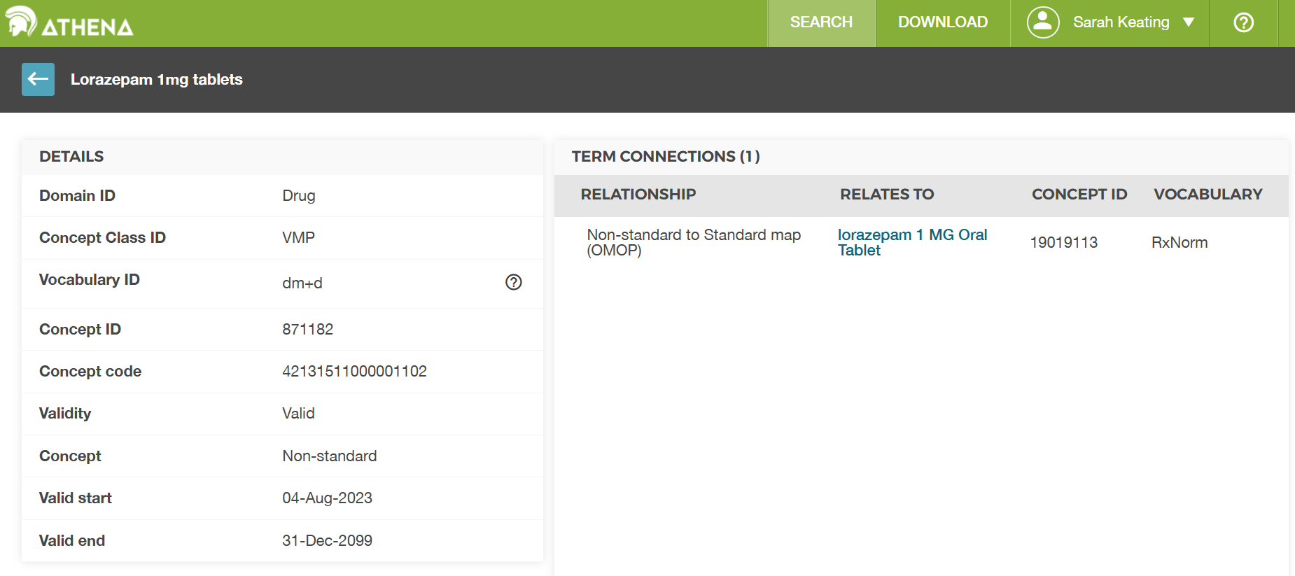
Looking at the entry for concept_id
871182 we can see that it is in the dm+d vocabulary. We
can see that is connected to the RxNorm concept “lorazepam 1 MG Oral
Tablet” which has concept_id 19019113. So
our assumption above was correct, but the concept table in our dataset
didn’t fill in the name fully so we couldn’t be sure without looking it
up in the official table.
TO TO: We need an example on quantity and route of administration to show how these are stored in the drug_exposure table and how they can be looked up in the concept table.
- Know that exposure of a patient to medications is mainly stored in the drug_exposure table
- Understand that drug concepts can be at different levels of granularity
- Understand that source values are mapped to a standard vocabulary
Content from Dates and times
Last updated on 2026-02-08 | Edit this page
Overview
Questions
- What
Objectives
- 1
Introduction
This episode considers dates and times in the OMOP Common Data Model (CDM).
For this episode we will be using a sample OMOP CDM database that is pre-loaded with data. This database is a simplified version of a real-world OMOP CDM database and is intended for educational purposes only.
(UCLH only) This will come in the same form as you would get data if you asked for a data extract via the SAFEHR platform (i.e. a set of parquet files).
As part of the setup prior to this course you were asked to download
and install the sample database. If you have not done this yet, please
refer to the setup instructions provided earlier in the course. For now,
we will assume that you have the sample OMOP CDM database available on
your local machine at the following path:
workshop/data/public/ and the functions in a folder
workshop/code.
You will then need to load the database as shown in the previous episode.
R
open_omop_dataset <- function(dir) {
  open_omop_schema <- function(path) {
    # iterate table level folders
    list.dirs(path, recursive = FALSE) |>
      # exclude folder name from path
      # and use it as index for named list
      purrr::set_names(~ basename(.)) |>
      # "lazy-open" list of parquet files
      # from specified folder
      purrr::map(arrow::open_dataset)
  }
  # iterate top-level folders
  list.dirs(dir, recursive = FALSE) |>
    # exclude folder name from path
    # and use it as index for named list
    purrr::set_names(~ basename(.)) |>
    purrr::map(open_omop_schema)
}
R
omop <- open_omop_dataset("./data/")
and the useful functions we created in the previous episode to look up concept names/ids.
R
library(arrow)
library(dplyr)
get_concept_name <- function(id) {
  omop$public$concept |>
    filter(concept_id == !!id) |>
    select(concept_name) |>
    collect()
}
R
get_concept_id <- function(name) {
  omop$public$concept |>
    filter(concept_name == !!name) |>
    select(concept_id) |>
    collect()
}
Dates and times in OMOP
Dates and times are used in most tables to record when events
happened,usually where they start and end date recorded. In many places
there is also a time component, for example to record the time of day
when a measurement was taken. Column names are frequently either
suffixed with _date or _datetime to indicate
whether they contain just a date or both date and time information.
However in our dataset dates and times are recorded as strings rather
than as date or datetime objects. This is because the parquet files
don’t have a standard way to store date and datetime objects, so they
are stored as strings in the format “YYYY-MM-DD” for dates and
“YYYY-MM-DD HH:MM:SS” for datetimes. When we read the data into R, we
can convert these strings to date or datetime objects using the
as.Date() or as.POSIXct() functions,
respectively. This will allow us to perform date and time calculations
and visualizations more easily.
Usually the dates come in pairs, for example
condition_start_date and condition_end_date in
the condition_occurrence table. This allows us to determine
the duration of a condition, for example, by calculating the difference
between the start and end dates.
Challenge
Using the condition_occurrence table, find the average
duration of conditions in this dataset.
R
# First we need to read in the condition_occurrence table
condition_occurrence <- omop$public$condition_occurrence |>
    collect()
# Then we need to exclude any rows where the end date is missing, as we can't calculate the duration for these
condition_occurrence <- condition_occurrence |>
    filter(!is.na(condition_end_date))
# Now we can calculate the duration of each condition by taking the difference between the end date and the start date

# TWO DO:fix this
condition_occurrence <- condition_occurrence |>
  mutate(condition_duration = as.numeric(as.Date.numeric(condition_end_date) - as.Date.numeric(condition_start_date)))
ERROR
Error in `mutate()`:
ℹ In argument: `condition_duration =
  as.numeric(as.Date.numeric(condition_end_date) -
  as.Date.numeric(condition_start_date))`.
Caused by error in `unclass(x) * 86400`:
! non-numeric argument to binary operator
R
average_duration <- mean(condition_occurrence$condition_duration, na.rm = TRUE)
average_duration
OUTPUT
[1] NAIt is not uncommon for the end date to be missing in the data, for example if a condition is ongoing at the time of data extraction. In this case, we can only calculate the duration for conditions that have an end date recorded.
Also consider the measurement table where we have both a
measurement_date and a measurement_datetime
column. The measurement_date column contains just the date
of the measurement, while the measurement_datetime column
contains both the date and time of the measurement. Depending on the
analysis we want to do, we may choose to use one or the other of these
columns. Note generally a measurement doesn’t have a start and end date,
but just a single date or datetime when the measurement was taken.
Challenge
Using the measurement table, graph the
Body temperature of patient 113over time. You
can use either the measurement_date or
measurement_datetime column for the x-axis.
R
library(ggplot2)
# First we need to know the concept id for body temperature
get_concept_id("Body temperature")
OUTPUT
# A tibble: 1 × 1
  concept_id
       <int>
1    3020891
R
# Then we need to read in the measurement table, filter for the measurements of interest and collect the data into memory
measurement <- omop$public$measurement |>
    filter(person_id == 1113 & measurement_concept_id == 3020891) |>
    collect()
# Now we can plot the body temperature over time
ggplot(measurement, aes(x = measurement_datetime, y = value_as_number)) +
    geom_line() +
    geom_point() +
    labs(title = "Body temperature of patient 113 over time",
         x = "Date and time of measurement",
         y = "Body temperature (°C)")
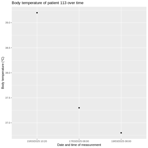
Dates and times are used in most tables in the OMOP CDM to record when events happened.
They are often used in pairs to record the start and end of an event, which allows us to calculate the duration of that event.